Exploring the design of a temperature probe with dimension reduction
In many engineering design tasks, we suffer from the curse of dimensionality. The number of design parameters quickly becomes too large for us to effectively visualise or explore the design space. We could attempt to use a design optimisation procedure to arrive at an “optimal” design, however, the curse of dimensionality places a computational burden on the cost of the optimisation. Also, in many cases we wish to understand the design space, not just spit out a “better” design.
This brings us to dimension reduction, a set of ideas which allows us to reduce high dimensional spaces to lower dimensional ones. By reducing the design space to a small number of dimensions, we can more easily explore it, allowing for:
- A better physical understanding.
- Exploration of previously unexplored areas of the design space.
- Obtaining new “better” designs.
- Assessing sensitivity to manufacturing uncertainties.
This post summarises our recent ASME Turbo Expo 2020 paper, where we use equadratures to perform dimension reduction on the design space of a stagnation temperature probe used in aircraft jet engines.
Part 1: Obtaining dimension reducing subspaces
The probe’s design space
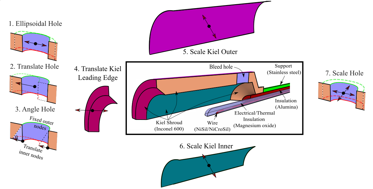
The temperature probe considered is shown in Figure 1. The probe design is parameterised by the seven design parameters, so our input design vector lies in a 7D design space $\mathbf{x} \in \mathbb{R}^7$.
Probes such as this are used in aero engines to measure the stagnation temperature in the flow. Ideally, we wish to bring the flow to rest isentropically, so that the temperature measured at the thermocouple $T_m$ is equal to the stagnation temperature $T_0$. However, in reality, various error sources mean the probe’s recovery ratio $R_r=T_m/T_0$ is always less than one.
In the paper we consider two design objectives:
-
To reduce measurement errors, we attempt to minimise the recovery ratio’s sensitivity to Mach number $\partial R_r/\partial M$.
-
To reduce the probe’s contamination of the surrounding flow, we wish to minimise the probe’s pressure loss coefficient $Y_p = (P_{0,in}-P_{0,out})/(P_{0,in}-P_{out})$, averaged across the Mach number range.
Both of these design objectives, $O_{R_r}$ and $O_{Y_p}$, are a function of our 7D design space $\mathbf{x}$:
\[O_{Y_p} = g(\mathbf{x}) \\ O_{R_r} = f(\mathbf{x})\]Design of experiment
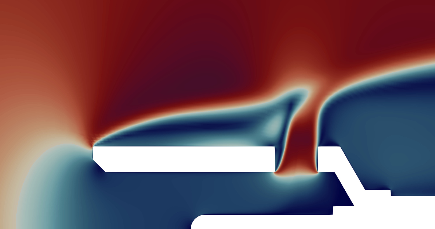
Before we can do any dimension reduction, we need some data! To sample the design space, 128 designs are drawn uniformly within the limits of the design space (using Latin hypercube sampling). These are meshed using @bubald’s great mesh morphing code, and put through a CFD solver (at 6 different Mach numbers). We end up with 128 different unique design vectors $\mathbf{x}$, and we post process the 768 CFD results to obtain 128 values of $O_{Y_p}$ and $O_{R_r}$.
Dimension reduction via variable projection
As before, let $\mathbf{x} \in \mathbb{R}^{d}$ (with $d=7$) represent a sample within our design space $\chi$ and within this space let $f \left( \mathbf{x} \right)$ represent our aerothermal functional, which could be either $O_{Y_{p}}\left( \mathbf{x} \right) $ or $O_{R_{r}}\left( \mathbf{x} \right) $. Our goal is to construct the approximation
\[f \left( \mathbf{x} \right) \approx h \left( \mathbf{U}^{T} \mathbf{x} \right),\]where $\mathbf{U} \in \mathbb{R}^{d \times m}$ is an orthogonal matrix with $m \ll d$, implying that $h$ is a polynomial function of $m$ variables—ideally $m=1$ or $m=2$ to facilitate easy visualization. In addition to $m$, the polynomial order of $h$, given by $k$, must also be chosen. The matrix $\mathbf{U}$ isolates $m$ linear combinations of all the design parameters that are deemed sufficient for approximating $f$ with $h$. equadratures possesses two methods for determining the unknowns $\mathbf{U}$ and $h$; the method=active-subspace uses ideas from [1] to compute a dimension-reducing subspace with a global polynomial approximant, whilst method=variable-projection [2] solves a Gauss-Newton optimisation problem to compute both the polynomial coefficients and its subspace. Both of these methods involve finding solutions to the non-linear least squares problem
where $\boldsymbol{\alpha}$ represents unknown model variables associated with $h$. In practice, to solve this optimization problem, we assemble the $N=128$ input-output data pairs
\[\mathbf{X}=\left[\begin{array}{c} \mathbf{x}_{1}^{T}\\ \vdots\\ \mathbf{x}_{N}^{T} \end{array}\right], \; \; \; \; \mathbf{f}=\left[\begin{array}{c} f_{1}\\ \vdots\\ f_{N} \end{array}\right],\]and replace $f \left( \mathbf{x} \right)$ in the least squares problem above with the evaluations $\mathbf{f}$. To do this in *equadratures it is as simple as doing:
1
2
3
4
5
6
7
8
m_Y = 1  # Number of reduced dimensions we want
k_Y = 1 #Polynomial order

# Find a dimension reducing subspace for OYp
mysubspace_Y = Subspaces(method='variable-projection', sample_points=X, sample_outputs=OYp, polynomial_degree=k_Y, subspace_dimension=m_Y)

# Get the subspace Poly for use later
subpoly_Y = mysubspace_Y.get_subspace_polynomial()
There remains the question of what values to choose for the number of reduced dimensions $m$ and the polynomial order $k$. This is problem dependent, but a simple grid search is usually sufficient here. This involves looping through different values i.e. $m=[1,2,3]$ and $k=[1,2,3]$, evaluating the quality of the resulting dimension reducing approximations, and choosing values of $k$ and $m$ which give the best approximations. To quantify the quality of the approximations we used adjusted $R^2$ (see here), which can be calculated with the score helper function in equadratures.datasets:
1
2
OYp_pred = subpoly_Y.get_polyfit(X)
r2score = score(OYp, OYp_pred, 'adjusted_r2', X)
Note: We measure the $R^2$ scores on the training data here, i.e. the $N=128$ designs we used to obtain the approximations. This is OK in this case since we have only gone up to $k=3$ so we’re not too concerned with overfitting. If you were to try higher Polynomial orders it would be important to split the data into train and test data, and examine the $R^2$ scores on the test data to judge how well the approximations generalise to data not seen during training.
The subspaces
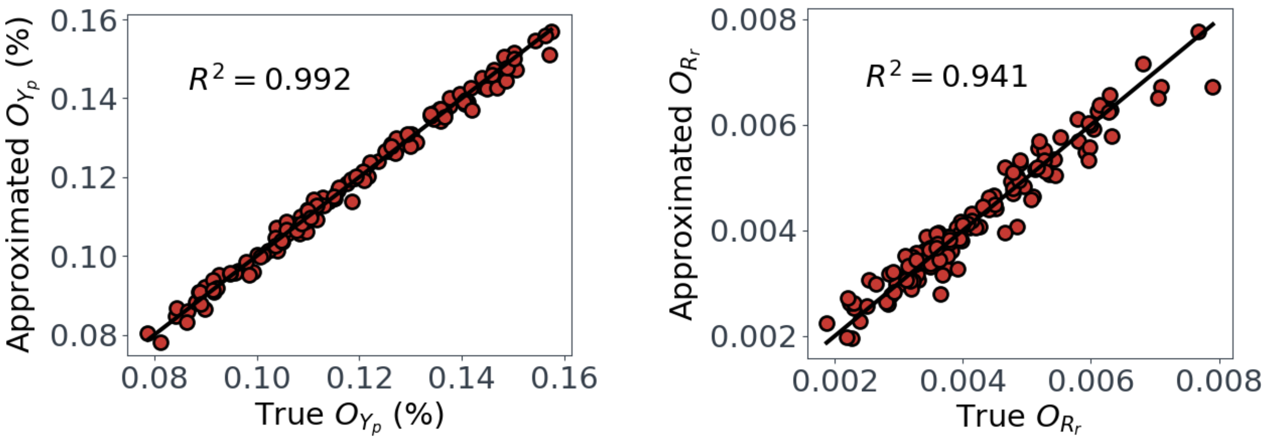
Upon performing a grid search for $O_{Yp}$ and $O_{Rr}$, we find $k,m=1$ are sufficient for $O_{Yp}$, but $k=3, m=2$ are required for $O_{Rr}$. With these values, we can see in Figure 3 that we get relatively good approximations for $O_{Yp}$ and $O_{Rr}$.
Now for the exciting part! The actual dimension reducing subspaces! A sufficient summary plot for $O_{Y_p}$, which summarises its behaviour in its reduced dimensional space, can easily be obtained from the mysubspace_Y object from earlier:
1
2
3
4
5
6
7
8
9
10
11
12
13
14
15
16
# Get the subspace matrix U
W_Y = mysubspace_Y.get_subspace()
U_Y = W[:,0:m_Y]

# Get the reduced dimension design vectors u=U^T.x
u_Y = X @ U_Y

# Plot the training data points on the dimension reducing subspace
plt.scatter(u_Y, OYp, s=70, c=OYp, marker='o', edgecolors='k', linewidths=2, cmap=cm.coolwarm, label='Training designs')

# Plot the subspace polynomial
u_samples = np.linspace(np.min(u_Y[:,0]), np.max(u_Y[:,0]), 100)
OYp_poly = subpoly_Y.get_polyfit( u_samples )
plt.plot(u_samples, OYp_poly, c='C2', lw=3, label='Polynomial approx.')
plt.legend()
plt.show()
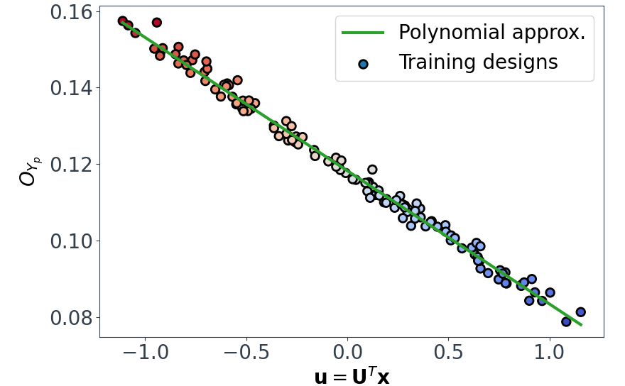
This shows that we have successfully mapped the original 7D function $O_{Y_p} = g(\mathbf{x})$ onto a 1D subspace $\mathbf{u}_Y = \mathbf{U}_Y^{T} \mathbf{x}$, and in this case $O_{Y_p}$ varies linearly with $\mathbf{u}_{Y}$.
Following a similar approach, but this time for the 2D $O_{R_r}$ subspace, gives us the summary plot shown in Figure 5. This one is especially interesting. $O_{R_r}$ appears to vary quadratically in one direction, with a clear minimum around $u_{R,1}\approx1$, while it decreases relatively linearly in the second direction $u_{R,2}$.
1
2
3
4
5
6
7
8
9
10
11
12
13
14
15
16
17
18
19
20
21
22
23
24
25
m_R = 2  # Number of reduced dimensions we want
k_R = 3 #Polynomial order

# Find a dimension reducing subspace for ORr
mysubspace_R = Subspaces(method='variable-projection', sample_points=X, sample_outputs=ORr, polynomial_degree=k_R, subspace_dimension=m_R)
subpoly_R = mysubspace_R.get_subspace_polynomial()
W_R = mysubspace_R.get_subspace()
U_R = W[:,0:m_R]
u_R = X @ U_R

# Plot the training data as a 3d scatter plot
figRr = plt.figure(figsize=(10,10))
axRr = figRr.add_subplot(111, projection='3d')
axRr.scatter(u_R[:,0], u_R[:,1], ORr,  s=70, c=ORr, marker='o', ec='k', lw=2)

# Plot the Poly approx as a 3D surface
N = 20
ur1_samples = np.linspace(np.min(u_R[:,0]), np.max(u_R[:,0]), N)
ur2_samples = np.linspace(np.min(u_R[:,1]), np.max(u_R[:,1]), N)
[ur1, ur2] = np.meshgrid(ur1_samples, ur2_samples)
ur1_vec = np.reshape(ur1, (N*N, 1))
ur2_vec = np.reshape(ur2, (N*N, 1))
samples = np.hstack([ur1_vec, ur2_vec])
ORr_poly = subpoly_R.get_polyfit(samples).reshape(N, N)
surf = axRr.plot_surface(ur1, ur2, ORr_poly, rstride=1, cstride=1, cmap=cm.gist_earth, lw=0, alpha=0.5)
That brings us to the end for now! In the second part of this post, I’ll demonstrate how these dimension reducing subspaces can actually be used.
Part 2: Using the dimension reducing subspaces
Physical insights
In Figure 4, we saw that $O_{Yp}$ is a linear function of its dimension reducing subspace $\mathbf{u}_Y=\mathbf{U}_Y^T\mathbf{x}$. In other words, each $j^{th}$ design has its own value of ${u_Y}_j \in \mathbb{R^1}$, which we can obtain by multiplying its oriignal design vector $\mathbf{x}_j\in \mathbb{R}^7$ by $\mathbf{U}_Y \in \mathbb{R}^{7\times1}$. The matrix $\mathbf{U}_Y$ (or vector in this case) gives us information on how the components of $\mathbf{x}$ (i.e. the original 7 design variables) move us around the $\mathbf{u}_Y$ subspace:
\[\mathbf{U}_{Y} =[0.05,0.01,\overbrace{-0.12}^{\text{Angle hole}},-0.02,\overbrace{0.98}^{\text{Kiel }\oslash_{outer}},0.02,\overbrace{0.17}^{\text{Hole }\oslash}]\]For example, The 0.98 for the Kiel outer diameter, tells us that increasing this design parameter will significantly increase $\mathbf{u}_Y$, and as Figure 4 shows, decrease $O_{Yp}$. On the other hand, the very small numbers for other elements of $\mathbf{U}_Y$ implies that varying these design parameters will have almost no impact on $\mathbf{u}_Y$ (and therefore $O_{Yp}$).
Physically, it makes sense that increasing the Kiel outer diameter increases $O_{Yp}$, as much of the pressure loss is arising from the bluff body pressure drag effect of the probe, and this gets worse as the probe diameter is increased. The above set of ideas can also provide less obvious physical insights though. For example, consider the $O_{Rr}$ subspace, viewed from above:
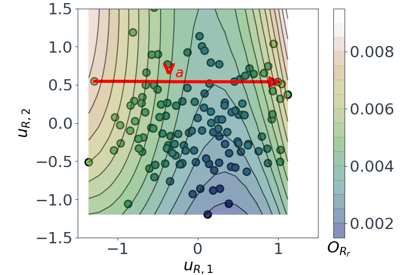
Its no longer as simple as looking at what components of $\mathbf{x}$ move us from left to right, as we’re in 2D now. Instead, we must choose what direction to move in. i.e. let’s take the direction $\mathbf{v}_a$ shown in Figure 6. If we look at the components of the vector-matrix product $\mathbf{v}_a \mathbf{U}_R$ (where $\mathbf{U}_R \in \mathbb{R}^{7\times 2}$ is the subspace matrix for $O_{Rr}$):
1
2
3
4
5
6
7
8
9
10
# Define va as a vector between two designs
va = u_R[112,:] - u_R[58,:]

# Normalise va
va /= np.sqrt(np.sum(va*va))

# Take product va*Ur
prod = va[0]*U_R[:,0] + va[1]*U_R[:,1]

# and then plot bar chart showing components of va...
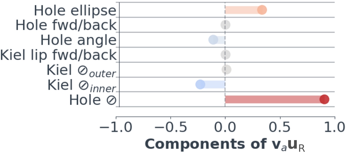
This tells us how elements in $\mathbf{x}$ move us along the vector $\mathbf{v}_a$. For example, increasing the vent hole diameter moves us forward along $\mathbf{v}_a$, whilst increasing the Kiel inner diameter moves us in the reverse direction. In the paper, we go into more detail about what physical insights such as these can tell us about the probe’s design space.
Obtaining new designs
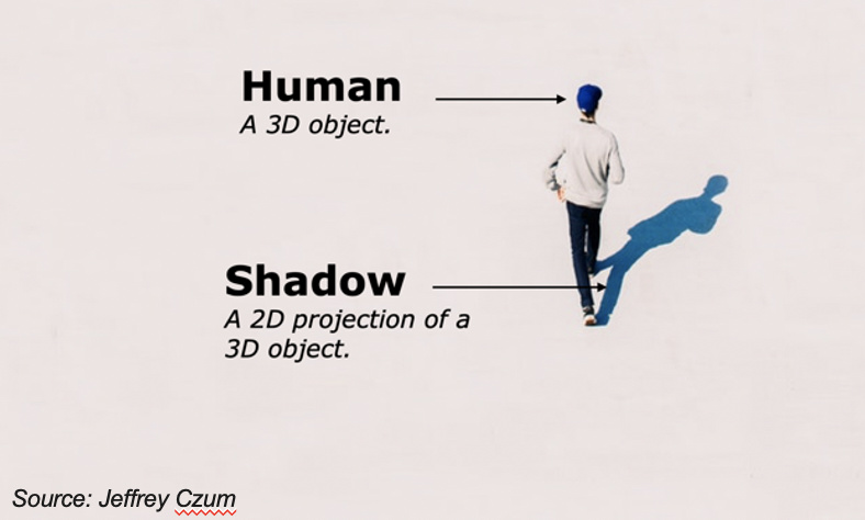
Before looking at finding new designs, its valuable to consider the bounds of the current design space. Our design vectors $\mathbf{x}_j$ can be considered to lie in a 7 dimensional hypercube
\[\chi \subset [-1,1]^7 \;\;\; \text{where} \;\;\; \mathbf{x}_j \in \chi \;\;\; \text{for} \;\;\; j=1,\dots,N,\]Similar to the way a human (a 3D object!) projects a 2D shadow on the ground, our 7D hypercube projects a 2D silhouette onto the 2D $O_{Rr}$ subspace (thanks to @psesh for the analogy!).
This 2D projection of the design space is referred to as the zonotope, and can be obtained from equadratures with the .get_zonotope_vertices() method. Below this is plotted, along with contours of $O_{Rr}$.
1
2
3
4
5
6
7
8
9
10
11
12
13
14
15
16
17
18
# Plot zonotope for Rr (the black line)
zone_R = mysubspace_R.get_zonotope_vertices()
zone_R = polar_sort(zone_R) # polar_sort function available on request
plt.plot(np.append(zone_R[:,0],zone_R[0,0]), np.append(zone_R[:,1],zone_R[0,1]),'k-',lw=3)

# Plot color contours of ORr (within the convex hull of the current u_R samples)
# The grid_within_hull function uses scipy.spatial.ConvexHull to find the convex hull
# of the given points (available upon request).
new_samples = grid_within_hull(u_R, N=25)
ORr_values = subpoly_R.get_polyfit(new_samples)
cont = plt.tricontourf(new_samples[:,0], new_samples[:,1], ORr_values, alpha=0.8, levels = 20, cmap=cm.gist_earth)
plt.tricontour(new_samples[:,0], new_samples[:,1], ORr_values, alpha=0.5, levels=20, colors='k')

# Plot baseline design location and direction of new design
plt.plot(uRbaseline[0],uRbaseline[1], 'oC3', ms=15, mfc='none', mew=3)
unew = [0.4,-1.4]
vnew = unew - u2baseline
plt.arrow(u2baseline[0], u2baseline[1], vnew[0], vnew[1])
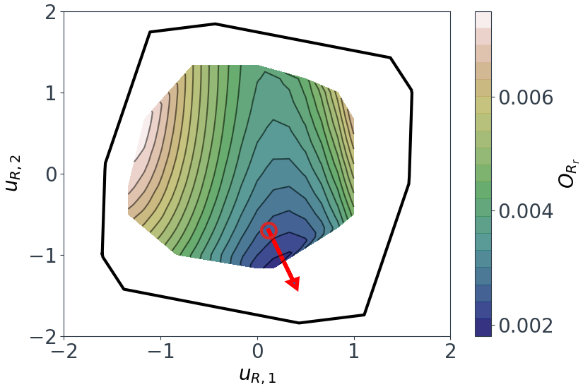
The contours of $O_{Rr}$ are only plotted within the convex hull of the training data. In other words, the contours are only plotted in the region of the design space covered by our CFD simulations. This is eye opening, although our DoE uniformly sampled throughout the region $\chi \subset [-1,1]^7$, there are still large areas of the design space which are completely unexplored!
It follows that we can use the above plot to discover new designs in unexplored regions of the design space. The baseline design is highlighted by the red circle in Figure 9. It looks like we might be able to lower $O_{Rr}$ even further by heading off in the direction of the red arrow. We can pick a new point e.g. $\mathbf{u}_{R,new} = (0.4,-1.4)$, and generate new design vectors $\mathbf{x}_{new}$ there:
1
2
3
4
# Generate 10 new xnew vectors for the chosen unew vector
# xnew has dimensions (10,7)
unew = [0.4,-1.4]
xnew = mysubspace_R.get_samples_constraining_active_coordinates(10,unew)
There are an infinite number of $\mathbf{x}$ vectors which can be transformed to a single $\mathbf{u_R}$ vector. Therefore, when finding $\mathbf{x}$ for a given $\mathbf{u_R}$, the .get_samples_constraining_active_coordinates() method will rapidly generate as many unique $\mathbf{x}$ design vectors as we want. You could generate 100 (or 10000!) designs, and select a design according to other design constraints. In the paper we use the $O_{Yp}$ approximation to quickly approximate $O_{Yp}$ for each of the new designs, and then choose designs which minimise both design objectives together. Please ask if you’d like the code used to do this step!
Sensitivity to manufacturing uncertainty
So far, we’ve been trying to minimise $O_{Rr}=\partial R_r/\partial M$, the sensitivity of $R_r$ with respect to Mach number. For real probes, manufacturing tolerances might mean it’s also important to minimise the sensitivity of $R_r$ with respect to the input design vector $\mathbf{x}$. One approach to understanding the sensitivities is to fit a polynomial in the full 7D design space, and then compute Sobol indices (see @Nick’s post https://discourse.effective-quadratures.org/t/sensitivity-analysis-with-effective-quadratures/30).
1
2
3
4
5
6
7
8
9
10
11
12
13
14
15
16
# Construct a Poly for Rr (at Mach=0.8)
 s = Parameter(distribution='uniform', lower=-1., upper=1., order=2)
myparams = [s for _ in range(0, dim)]
mybasis = Basis('total-order')
mypoly = Poly(parameters=myparameters, basis=mybasis, method='least-squares', sampling_args= {'mesh': 'user-defined', 'sample-points': X, 'sample-outputs': Rr})
mypoly.set_model()

# Check R2
Rr_pred = mypoly.get_polyfit(X)
r2score = score(Rr, Rr_pred, 'adjusted_r2', X)

# Get Sobol indices
Si = mypoly.get_sobol_indices(order=1)
Sij = mypoly.get_sobol_indices(order=2)

# Plot...
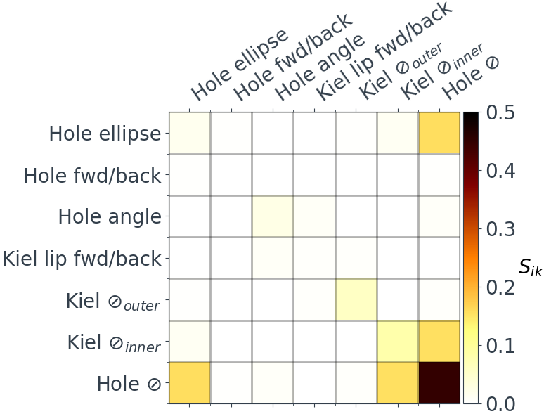
This is certainly informative, for example, we can see that $R_r$ is most sensitive to the hole diameter, followed by the Kiel inner diameter and hole ellipse. If want to limit uncertainty in $R_r$, and therefore the measured $T_0$, we need to have tight controls on the manufacturing tolerances of these parameters.
With dimension reduction we can go much further though! To explore this, we construct another dimension reducing approximation for $R_r$ itself (at Mach=0.8):
\[R_r \left(\mathbf{x}_j \right) \approx \hat{g} \left(\hat{\mathbf{U}}^T \mathbf{x}_j \right)\]In this case we are concerned with the sensitivity of $R_r$ to perturbations in the design parameters:
\[R_r \left( \mathbf{x}_j + \Delta \right) \approx \hat{g} \left( \hat{\mathbf{U}}^T \left( \mathbf{x}_j + \Delta \right) \right)\]where $\Delta$ represents manufacturing variations injected into each design parameter. The $R_r$ subspace is shown in Figure 11 (left). The arrows demonstrate the influence of perturbing each parameter individually by $\Delta=0.1$. Perturbations are applied to the baseline design, but the decomposition
\[\hat{\mathbf{U}}^T \left( \mathbf{x}_j + \Delta \right) = \hat{\mathbf{U}}^T \mathbf{x}_j + \hat{\mathbf{U}}^T\Delta\]proves that the arrows will be the same anywhere in the $R_r$ subspace (the $\hat{\mathbf{U}}^T\Delta$ term is not a function of $\mathbf{x}_j$). Comparing the magnitude of the arrows indicates what design parameters cause the most significant movement in the $R_r$ subspace. Additionally, by also considering the contours of $R_r$, the arrows indicate what parameters are important for a given design.
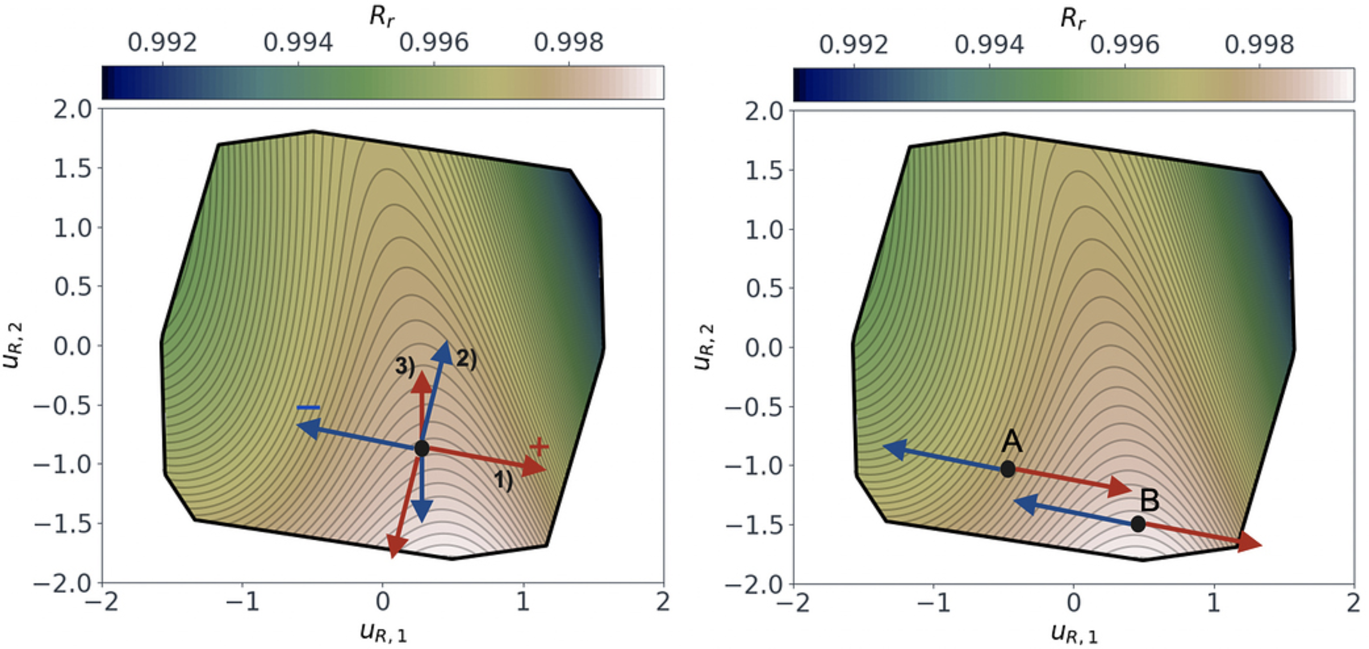
These plots can also be used to find designs which are insensitive to a certain design parameter. For example, imagine the factory reports that they are unable to tightly control the hole diameter when manufacturing a probe. We would want to find a probe design which minimises the design objectives, whilst having its $R_r$ relatively insensitive to the hole diameter. From Figure 11 (right), we see that designs at point B would be preferable over designs at A. Since, at point A, perturbations in the hole diameter run perpendicular to the $R_r$ iso-lines, while at B they run parallel.
Other Examples
For other examples of how the dimension reduction module in equadratures can be used, check out:
- Nicholas Wong’s great blog post, where he examines the use of dimension reduction for flowfield approximations.
- Pranay Seshadri’s paper, introducing dimension reducing turbomachinery performance maps.
- James Gross’ paper, where he combines dimension reduction ideas with trust region optimisation methods.
References
[1] Constantine, P. G. (2015). Active Subspaces. Society for Industrial and Applied Mathematics. Book.
[2] Hokanson, J. M., & Constantine, P. G. (2018). Data-Driven Polynomial Ridge Approximation Using Variable Projection. SIAM Journal on Scientific Computing, 40(3), A1566–A1589. Paper.