Uncertainty quantification of computational simulations

In this blog post, I’ll talk about using the equadratures python package for uncertainty quantification of computational simulations. If you’d like to follow along, the code from this post can be run interactively on the cloud by clicking below:

Uncertainty quantification

Uncertainty quantification (UQ) is the science of quantifying, and perhaps reducing, uncertainties in both computational and real world applications. Many fields of engineering rely on computational simulations, such as Computational Fluid Dynamics (CFD) simulations, to predict Quantities of Interest (QoI’s), such as lift and drag coefficients for an aerofoil or vehicle. These simulations have many sources of uncertainty, which can be broadly split into two categories:

• Aleatory uncertainties - statistical uncertainties, which area caused by intrinsic variability in our experiment or physical process. Examples of these would uncertainties in manufactured geometries or inflow conditions of the flow we are simulating.

• Epistemic uncertainties - systematic uncertainties, which are due to things one could in principle know but do not in practice. An example of this would be the uncertainty which arises due to the turbulence model used in a CFD simulation.

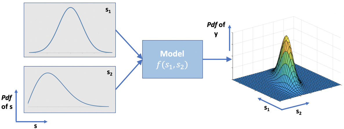
The effect of aleatory uncertainties on a QoI can be quantified by propagating these uncertainties through our computational model, as shown in Figure 1. Here $s_1$ and $s_2$ are our input parameters, which are represented with probability density functions (PDF’s) since there is some uncertainty in their definition. These parameter uncertainties will be propagated through the model $f(s_1,s_2)$, so that we obtain a PDF of our output quantity of interest $y$.

Figure 1: Forward propagation of two parameter uncertainties through a model.

Backward analysis (statistical inference) techniques can be used to do the opposite i.e. infer the $s_1$ and $s_2$ distributions from the measured distribution of $y$, however here we’ll stick to forward propagation. For a comprehensive review of statistical inference and quantification of epistemic uncertainties from turbulence models, check out this recent review paper [1].

Computing moments with polynomials vs random sampling

Before getting to forward propagation on a real CFD example, lets first explore the motivation for using equadratures for this, by comparing it to a random sampling approach. It is important to note that often we are not interested in the actual PDF of our QoI $y$, but only its statistical moments, the first four of which are shown in Figure 2. Here we will focus on the first two, the mean $\bar{y}$ and variance $Var(y)$, which often tell us sufficient information about the uncertainty in our QoI’s.

Figure 2: The first four statistical moments of a probability distribution.
Source: https://medium.com/paypal-engineering/statistics-for-software-e395ca08005d

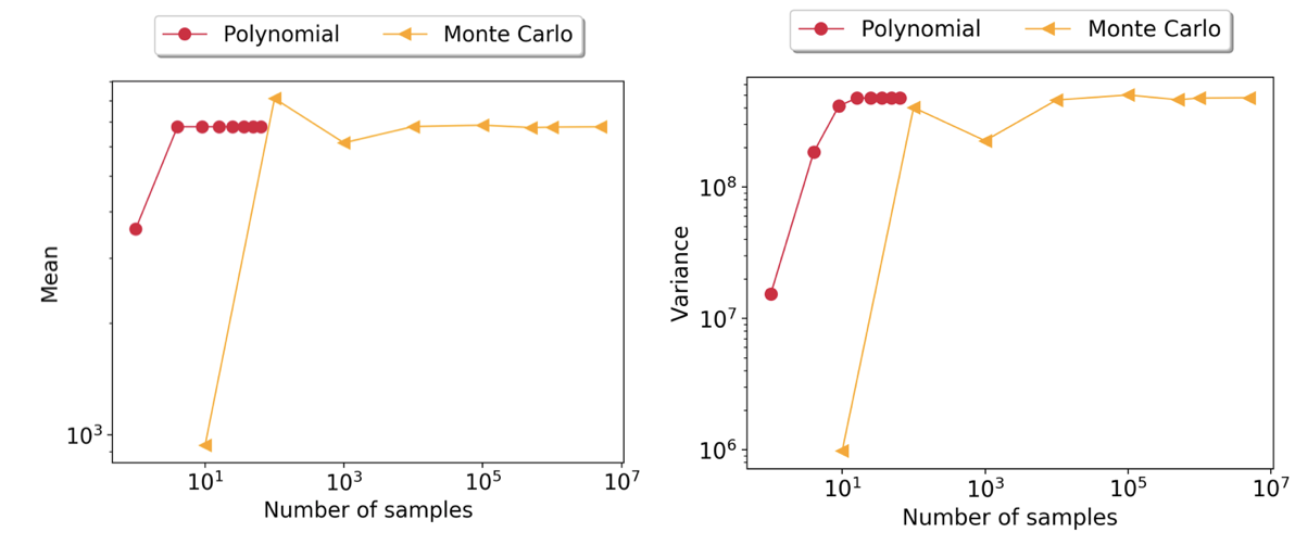
Why bother using polynomials for estimating moments? What exactly is the advantage? Moreover, are we guaranteed that we will converge to the Monte Carlo solution? The answer is a resounding yes! In fact, this is precisely what Dongbin Xiu and George Karniandakis demonstrate in their seminal paper [2]. @Nick explores this further in tutorial 4 for a 2D problem (Rosenbrock’s function), where he demonstrates the cost savings gained by using polynomials (see Figure 3!).

Figure 3: Mean and variance estimates versus number of samples for Monte Carlo type random sampling and polynomial approximations (with equadratures). Source.

In this post we will start with a more simple univariate problem. We have one input parameter $s_1$, which has a uniform distribution $\mathcal{S}=\mathcal{U}[0,1]$, and our model is a simple quadratic $f(s_1) = -s_1^2 + s_1 + 1$.

Figure 4: A simple univariate forward propagation example.

We wish to compute the mean and variance of $y=f(s_1)$ due to the uncertainty in $s_1$. As a reference, the analytical mean and variance of $y$ are:

\[\overline{f(s_1)} = \int_0^1{f(s_1)}ds_1=\frac{7}{6}= \mathbf{1.1\dot{6}}\] \[Var\left({f(s_1)}\right) = \int_0^1{f(s_1)^2}ds_1 - \overline{f(s_1)}^2=\frac{1}{180}= \mathbf{0.00\dot{5}}\]

Random sampling

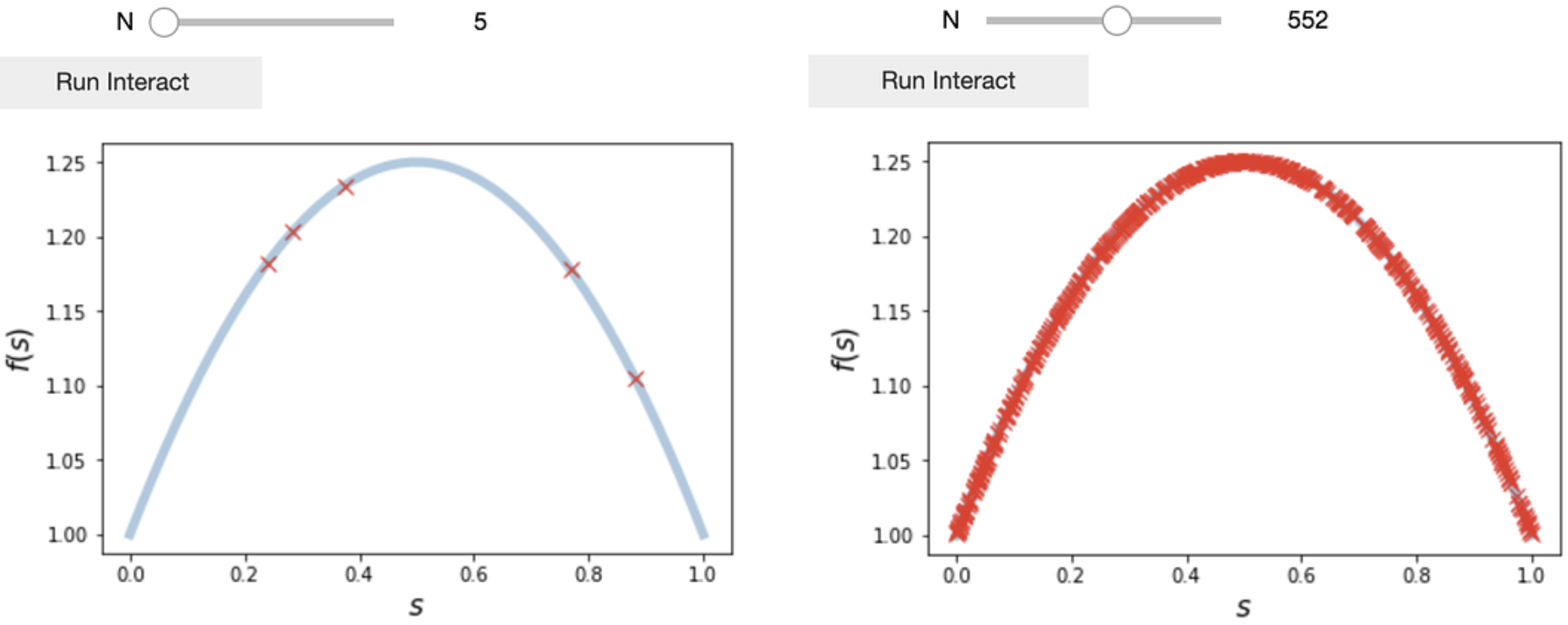
The most simple approach is a Monte Carlo type approach where we evaluate our model $f(s_1)$ at $N$ number of $s_1$ randomly sampled from $\mathcal{S}$. Then we calculate the mean and variance of the collected model outputs.

our_function = lambda s: -s**2 + s + 1 
s1_samples = np.random.uniform(low=0,high=1,size=N)
y_samples = f(s1_samples)
mean = np.mean(y_samples)
var = np.var(y_samples)

On the azure notebook version of this post there is an interactive widget where you can perform the above procedure for different $N$. You should find that a large number is required for $N$ before accurate moments are obtained, especially for the variance. This might be OK in this example, but not for a case where each model simulation is a CFD simulation requiring minutes/hours/days to run!

Figure 5: Random sampling of the model function $f(s_1)$ with $N=5$ and $N=552$.

Using equadratures

Alternatively, we can use equadratures to compute the moments of $y$, with the code below. We simply declare the usual building blocks (a Parameter, Basis and Poly object), give the Poly our data (or function) with set_model, and then run get_mean_and_variance.

s1 = Parameter(distribution='uniform', lower=0., upper=1., order=2)
mybasis = Basis('univariate')
mypoly = Poly(parameters=s1, basis=mybasis, method='numerical-integration')
mypoly.set_model(our_function)
mean, var = mypoly.get_mean_and_variance()

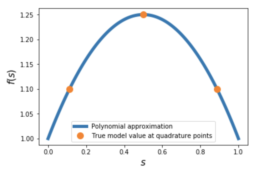
The accuracy is clearly pretty good! What have we actually done here? Behind the scenes, equadratures has calculated the quadrature points in $s_1$ (dependent on our choice of distribution, order and the Basis). Then it has evaluated our model at these points, and used the results to construct a polynomial approximation (response surface), $f(s_1)\approx \sum_{i=1}^N x_i p_i(s_1)$.

Figure 6: Polynomial approximation of the model $f(s_1)$, and the three quadrature points the model was evaluated at.

Once we have the polynomial coefficients $x_i$, it is straightforward to obtain the mean and variance: \(\mathbb{E}[f(s)]=\int_Sf(s)\omega(s)ds=x_0\)

\[\sigma^2[f(s)]=\int_Sf^2(s)\omega(s)ds-\mathbb{E}[f(s)]^2=\sum_{i=1}^N x_i^2\]

Since we selected order=2 here, we only required $N=3$ model evaluations to get exact values for the moments. This is expected since our model is a quadratic polynomial itself in this case. However, it still demonstrates the potential of this approach, compared to random sampling.

A CFD example!

Now we have seen the potential of using polynomial approximations to compute moments, we will explore a real CFD example, the von Karman Institute LS89 turbine cascade [3]. The open source SU2 CFD code is used for all simulations here.

Figure 7: RANS simulation of the VKI turbine cascade.

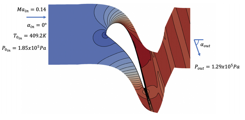
For the Reynolds-Averaged Navier-Stokes (RANS) turbulence model, we select the SST model. This is a 2-equation model, solving an equation for the turbulent kinetic energy $k$, and the specific dissipation rate $\omega$.

The addition of additional equations for $k$ and $\omega$ can improve accuracy compared to a 0- or 1-equation RANS model, but it adds an additional source of aleatory uncertainty; the specification of inflow boundary conditions for $k$ and $\omega$. We wish to estimate the uncertainty in our QoI due to this new uncertainty source. Our QoI here is the loss coefficient for the cascade:

\[Y_p = \frac{p_{0_{in}}-p_{0}}{p_{0_{in}}-p_{_{inflow}}}\]

SU2 uses turbulence intensity $Ti$, and turbulent viscosity ratio $\nu_t/\nu$ as its turbulent boundary conditions ($k = \frac{3}{2}(U \;Ti)$ and $\omega = \frac{k}{\nu}\left(\frac{\nu_t}{\nu} \right)^{-1}$). We can often estimate $Ti$ with some confidence, since it can be measured using a hot-wire probe. However, $\nu_t/\nu$ is physically more vague, and it is more of an unknown quantity. For this reason we set $Ti$ to have a gaussian distribution, while for $\nu_t/\nu$ we can only say it lies within a certain range, therefore we choose a uniform distribution. Then we declare a Basis and Poly as usual…

s1 = Parameter(distribution='uniform', lower=1.0, upper=100, order=3) #turb2lamviscosity
s2 = Parameter(distribution='Gaussian', shape_parameter_A=10, shape_parameter_B=5, order=3) #Ti
mybasis = Basis('tensor-grid')
mypoly = Poly(parameters=[s1,s2], basis=mybasis, method='numerical-integration')

This time running set_model is a little more involved, since our model is a CFD simulation instead of a simple polynomial function. We first ask equadratures for the quadrature points, and save them to disk.

pts = mypoly.get_points()
np.save('points_to_run.npy', pts)

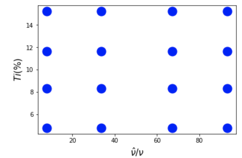
We have essentially just obtained a Design of experiments (DoE), telling us the turbulent inflow conditions to run our CFD at. This is straightforward to do, especially with the python scripting capability of SU2! Once this is done, we load the QoI ($Y_p$) from each simulation into a numpy array Y\_p, and give it to the Poly with mypoly.set_model(Yp). We can then compute the mean and variance.

mean, var = mypoly.get_mean_and_variance()

So our 95% confidence interval due to uncertainty in inflow turbulence specification is $Y_p\pm 0.00047$. This seems small but is actually 0.88% of the mean $Y_p$ value, so may be significant depending on your use case.

And there you have it! Quantification of aleatory uncertainties using equadratures, with far fewer model evaluations (CFD runs!) required compared to Monte Carlo approaches. These cost savings only increase as the number of parameters we wish to propagate increases!

Dealing with failed simulations

Any CFD practitioner is probably all too familiar with CFD simulations not converging! So what happens to the above in this case? In the companion notebook, we set a number of our DoE samples to NaN to explore this.

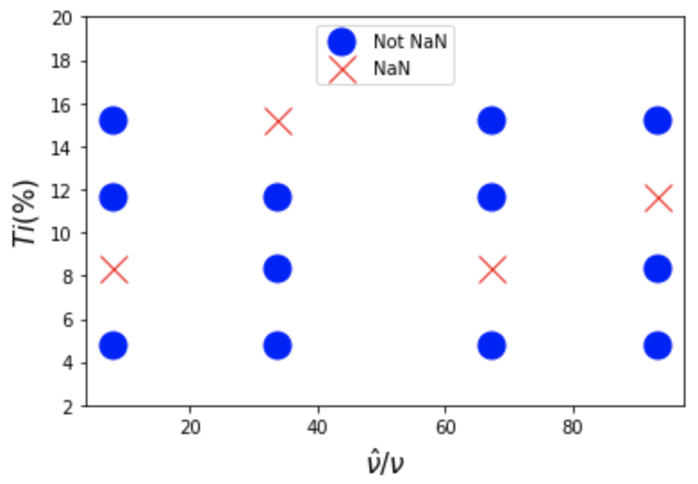
The answer is no problem! equadratures detects the NaN’s in our tensor-grid and automatically switches to a Least Squares technique to find the polynomial coefficients. The accuracy of the computed moments is within 2% of the previous values!

Sensitivity analysis

As a quick follow on from Nicholas Wong’s blog post over on our discourse, we can compute the Sobol’ indices for the above CFD polynomial approximation.

mypoly.get_sobol_indices(order=1)

Clearly, $Y_p$ is significantly more sensitive to $s_1$ ($\nu_t/\nu$) than $s_2$ ($Ti$). This is potentially a problem when we are looking to run CFD simulations of this nature, since ($\nu_t/\nu$) is more difficult to measure, so we often don’t have a good idea of what its value should be.

References

[1] Xiao, H., and Cinnella, P., (2019). Quantification of Model Uncertainty in RANS Simulations: A Review. Progress in Aerospace Sciences, 108. Preprint

[2] Xiu, D., and Karniandakis, G. E., (2002). The Wiener-Askey Polynomial Chaos for Stochastic Differential Equations. SIAM Journal on Scientific Computing, 24(2). Paper

[3] Segui, L. et al., (2017). LES of the LS89 cascade: influence of inflow turbulence on the flow predictions. Proceedings of 12th European Conference on Turbomachinery Fluid Dynamics & Thermodynamics. Paper